Introduction to mapSpainHist

mapSpainHist provides the municipal boundaries of Spain for each population census between 1900 and 2001, together with the figures of those censuses. This article shows how to get the maps, how to represent data on them and how to follow municipal changes over time.

Warning. The shape of most historical municipalities is an approximate reconstruction. The maps are useful above all to represent municipal data; use them with caution for geographic variables such as area or distances. See the methodology.

Installation and first load

remotes::install_github("pauvallprat/mapSpainHist")

library(mapSpainHist)
library(ggplot2)

The available censuses are:

mhist_census_years()
#>  [1] 1900 1910 1920 1930 1940 1950 1960 1970 1981 1991 2001

The function esp_get_munic_hist() returns an sf object with one polygon for each municipality in force at the given census. The first time it downloads the geometries from Zenodo (about 6.5 MB) and stores them in a local cache; afterwards it reads them directly from disk.

m1930 <- esp_get_munic_hist(1930)
nrow(m1930)
#> [1] 9343
head(sf::st_drop_geometry(m1930))
#>   cod_ine no_munic censo        municipio        prov cod_ccaa       ccaa
#> 1   01001        0  1930 Alegría-Dulantzi Araba/Álava       16 País Vasco
#> 2   01002        0  1930          Amurrio Araba/Álava       16 País Vasco
#> 3   01003        0  1930          Aramaio Araba/Álava       16 País Vasco
#> 4   01004        0  1930       Artziniega Araba/Álava       16 País Vasco
#> 5   01006        0  1930          Armiñón Araba/Álava       16 País Vasco
#> 6   01007        0  1930       Arrastaria Araba/Álava       16 País Vasco
#>        PJ hogares pder phec pob_serie
#> 1 Vitoria     146  810  735       810
#> 2 Vitoria     354 1595 1755      1595
#> 3 Vitoria     388 1945 1822      1945
#> 4 Vitoria     287 1108 1230      1108
#> 5 Vitoria      98  446  432       446
#> 6 Vitoria     122  680  655       680

Each row has the INE code of the municipality (cod_ine), the census figures (name, province, autonomous community, judicial district, households and de jure and de facto population) and the geometry. Non-municipal territories (common pastures, facerías, etc., with codes 53xxx) have no_munic = 1 and no census figures; they can be dropped with include_nonmunicipal = FALSE.

A population map

We represent the de jure population of each municipality in 1930. With moveCAN = TRUE the Canary Islands are placed next to the Peninsula, as the mapSpain package does. In this case it is advisable to draw the box that separates them too, with mapSpain::esp_get_can_box().

m1930 <- esp_get_munic_hist(1930, moveCAN = TRUE)
m1930$population <- cut(
  m1930$pder, c(0, 500, 1000, 2000, 5000, 20000, Inf), right = FALSE,
  labels = c("< 500", "500-999", "1,000-1,999", "2,000-4,999", "5,000-19,999", "20,000 or more")
)

ggplot(m1930) +
  geom_sf(aes(fill = population), colour = NA) +
  scale_fill_viridis_d(option = "magma", direction = -1, na.value = "grey85") +
  geom_sf(data = mapSpain::esp_get_can_box(), colour = "grey50") +
  labs(title = "De jure population by municipality, 1930", fill = "Inhabitants") +
  theme_void()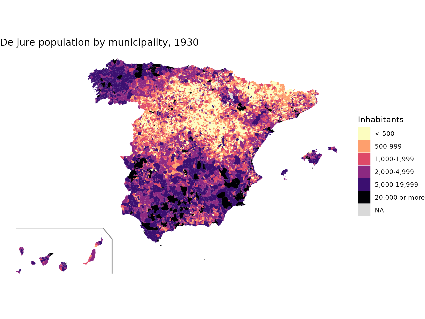

Municipalities throughout the 20th century

The censos table contains the figures of every municipality and every census between 1842 and 2011. A municipality is in force at a census when it has household figures (hogares). We can count how many municipalities there were at each census:

inforce <- censos[!is.na(censos$hogares) & censos$censo %in% mhist_census_years(), ]
table(inforce$censo)
#> 
#> 1900 1910 1920 1930 1940 1950 1960 1970 1981 1991 2001 
#> 9267 9262 9255 9262 9257 9214 9201 8653 8023 8076 8108

The sharp drop in the 1960s and 1970s corresponds to the municipal mergers of those years. As each map contains exactly the municipalities in force at its census, these changes can be followed on the ground. For example, Valdetórtola (Cuenca) was created in the 1970s from several municipalities and dissolved in the 1990s:

m81 <- esp_get_munic_hist(1981, epsg = 3035, census_data = FALSE)
area_vt <- sf::st_buffer(m81[m81$cod_ine == "16907", ], 12000)

maps <- lapply(c(1970, 1981, 1991), function(y) {
  m <- esp_get_munic_hist(y, epsg = 3035, census_data = FALSE)
  m <- m[lengths(sf::st_intersects(m, area_vt)) > 0, ]
  m$census <- y
  m
})
d <- do.call(rbind, maps)

ggplot(d) +
  geom_sf(aes(fill = cod_ine == "16907"), colour = "grey30", linewidth = 0.2) +
  scale_fill_manual(values = c(`FALSE` = "grey92", `TRUE` = "tomato"),
                    labels = c("Other municipalities", "Valdetórtola"), name = NULL) +
  facet_wrap(~census) +
  theme_void()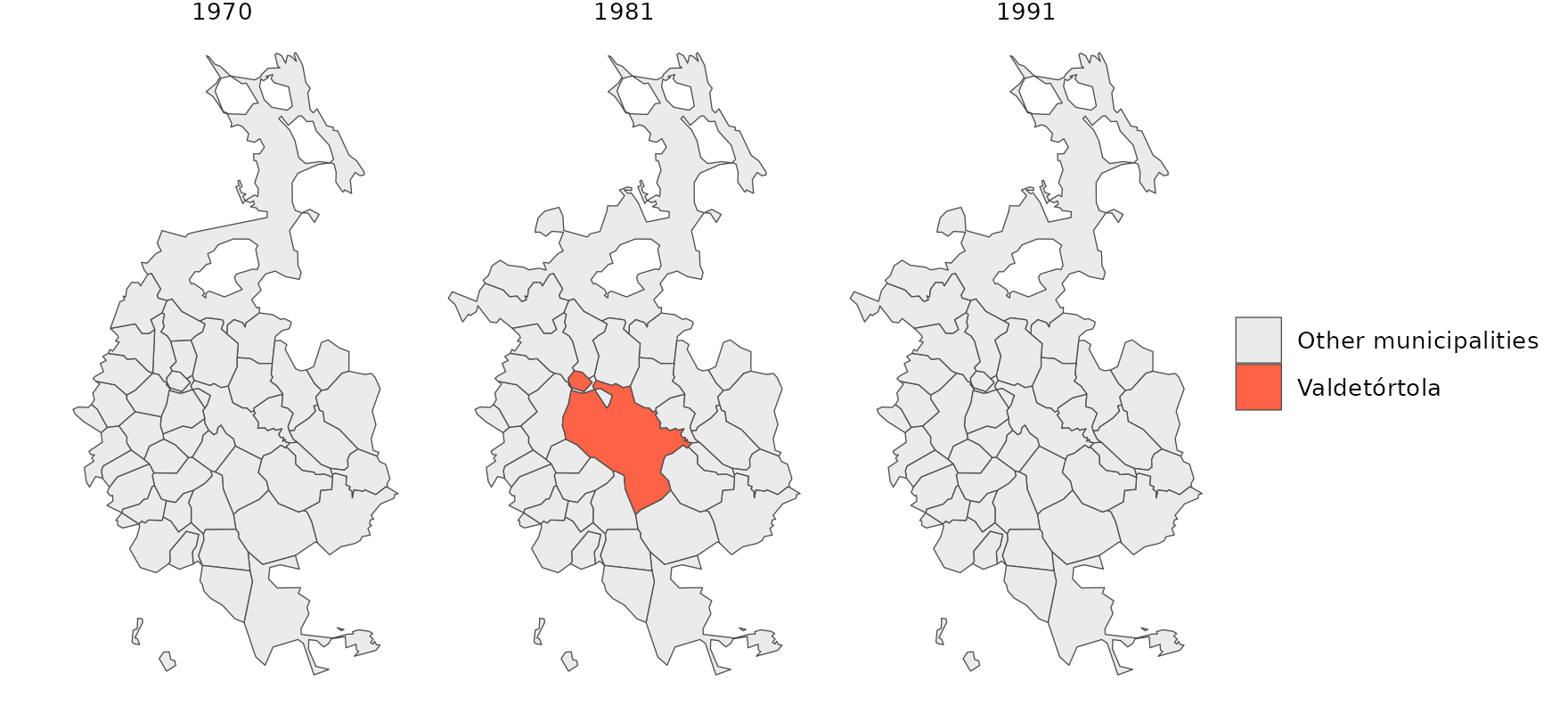

Adding your own data

To represent your own data (for example, election results or figures from another census), just join them by the INE code, cod_ine, a 5-character string:

mydata <- read.csv("municipal_data_1930.csv", colClasses = c(cod_ine = "character"))
m1930 <- merge(esp_get_munic_hist(1930), mydata, by = "cod_ine", all.x = TRUE)

To aggregate data to provinces, judicial districts or electoral districts, see the article Higher-level units and data aggregation.

Cache

The geometries are stored in the directory returned by mhist_cache_dir(). It can be changed for the session with mhist_set_cache_dir() or with the cache_dir argument of the functions, and emptied with mhist_clear_cache(). The argument update_cache = TRUE forces a new download.

mhist_cache_dir()
#> [1] "/home/runner/.cache/R/mapSpainHist"